The Time-Based Costs tool allows the user to calculate economic costs associated with the duration of flooding. This may be direct damages (eg to farm crops that after 3 days inundation, are unsalvageable), or may be indirect costs such as loss of business due to flooding.
Time-based costs can be calculated for all model results in the project, by integrating with information in point-based GIS datasets. Costs are calculated using Duration-Cost curves which relate the duration of floodwaters above the specified level to associated costs. Different cost curves can be used for the various objects in the GIS layer by linking each cost curve to an identifier in the GIS layer. The GIS layer must contain the following fields:
- critical level (the level above which the duration of "inundation" will be calculated)
- cost curve ID field (provides a cross reference to the duration-cost curve to use for each object in the layer - these may be grouped by specific object types)
Costs are calculated for each object by first determining the duration at which the water surface is above the critical level specified in the GIS layer, then finding which duration-cost curve to apply (from the cost cost curve ID field), and reading the cost value from the appropriate curve.
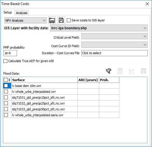
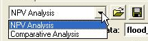
1) Select whether to do a Net Present Value (NPV) Analysis or a Comparative Analysis. A Comparative Analysis allows costs to be calculated for selected water surface layers. This facilitates a quick comparison of costs between different surfaces (eg differing flood mitigation options or magnitudes). An NPV Analysis will use selected water surface layers in the project (usually different probability events) to determine Average Annual Costs (AAC) and the NPV of this.
2) Select the GIS layer containing the property information for which to calculate time-based costs.
3) Select the fields in the GIS layer that define the critical level to determine the duration of inundation against.
4) Select the field in the GIS layer that defines the cost curve curve ID for each object in the layer. The values in this field must match the column headings of the cost curve .csv file.
5) Select the cost curve to use in the calculations by double clicking the edit box and locating the .csv file.
6) Select the water surface layers to calculate time-based costs for. For NPV analysis, you will also need to specify the Annual Recurrence Interval (ARI) or Annual Exceedance Probability (AEP) for each water surface. The default AEP assigned to the PMF event can be specified in the edit box. If your model results have been calculated in terms of an ARI, rather than an AEP, then the AEP is not simply 1/ARI, but rather using the following formula:![]() . This can be enforced by clicking the "Calculate True AEP for given ARI" option.
. This can be enforced by clicking the "Calculate True AEP for given ARI" option.
7) The Save costs to GIS layer tick box allows the user to specify whether the costs information should be saved as new fields in the GIS layer, or just displayed in the grid.
8) Click the Run Time-Based Costs button ![]() to calculate the costs.
to calculate the costs.
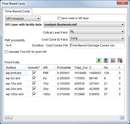
A summary of the time-based costs calculations are shown in the grid for each water surface. Total costs as well as the component costs for each cost curve category are displayed.
The summary can be saved to an external text file by clicking the Save time-based costs button ![]() .
.
(Available only for NPV Analysis)
Average Annual Costs provides an indication of the annual cost of flooding. It is calculated by determining the costs associated with various floods probabilities and then multiplying the costs by the likelihood of occurrence (ie calculating the area under the probability-cost curve), across the entire range of floods (i.e. from the $0 cost flood to the PMF). AAC can be grouped across all objects in the GIS layer or, if the results are saved to the GIS layer, provided on an individual object basis.
To commence an AAC calculation, click the Run Net Present Value Analysis button ![]() .
.
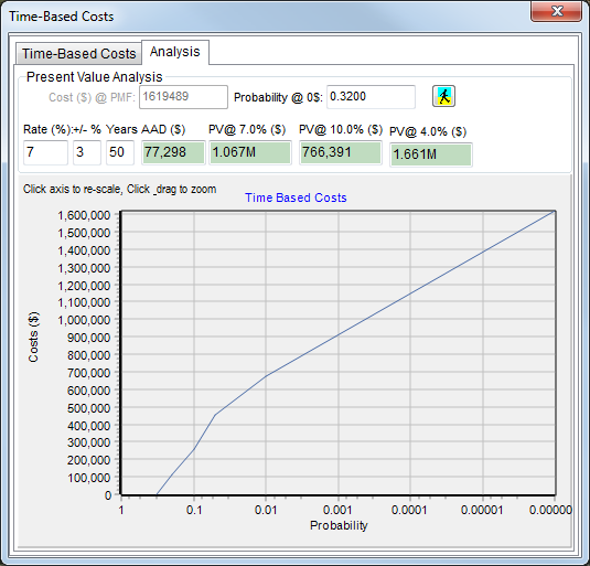
To calculate the AAC, the cost-probability curve (refer above figure) must be defined for the full range of flooding (i.e. from the flood that results in $0 costs, through to the PMF event). If it is not specified, the cost for the PMF event can be entered into the edit box at the top of the form. If not specified, the probability of the flood that results in zero costs can be entered into the edit box at the top of the form. The user may wish to extrapolate either of these values from the probability-cost curve. Double clicking the X-axis of the curve allows the user to specify/reset a new display range (zoom in).
Click the Run cost calcs button ![]() to calculate the AAD.
to calculate the AAD.
A Net Present Value Analysis can be carried out at the same time that the AAD is calculated. The Net Present Value analysis will discount the AAD (using a specified "discount rate") over a specified period to provide a total net present value. Such analysis may be useful in comparing the benefits of proposed flood mitigation works with the capital cost of constructing/implementing the works.
1) Specify the discount rate to use in the analysis.
2) Specify the high/low tolerance (+/-) on the discount rate. This provides ready sensitivity analysis.
3) Specify the duration to carry the net present value analysis over. This may be the design life of the structure.
Click the Run cost calcs button ![]() to calculate the AAC and Net Present Value. Note that the net present value is reported for the specified discount rate and the high/low tolerance discount rates.
to calculate the AAC and Net Present Value. Note that the net present value is reported for the specified discount rate and the high/low tolerance discount rates.
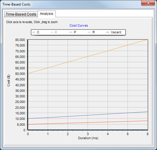
The duration-curve is a simple .csv file (which can be readily created in Excel). It provides the cost associated with various durations of inundation for any number of property types (cost curve ID). The first row contains the cost curve ID's. The first column contains the keyword "Duration", with subsequent columns containing the Cost Curve ID. These cost curve ID's must be exactly the same as the data in the Cost Curve ID field of the GIS layer.
In subsequent rows, the first column contains the duration of flooding. Each subsequent column contains the costs associated with that duration of inundation. A simple duration-curve is presented as a table below:
Duration,Crops,Loss Of Production,Pumping Costs,Management,No Cost
0,0,0,0,0,0
0.01,10000,50000,5000,200,0
1,11000,55000,5500,200,0
2,12000,60000,6000,200,0
3,13000,65000,6500,200,0
4,14000,70000,7000,200,0
5,15000,75000,7500,200,0
6,16000,80000,8000,200,0
In the above example, the Cost Curve ID field of the GIS layer would have values of either "Crops", "Loss Of Production", "Pumping Costs", "Management" or "No Cost", representing the different types of objects in the GIS layer.
The Duration-Cost curves can be plotted by clicking the Plot duration-cost curves button ![]() .
.